How to Analyze Polynomial Regression

SmartstatXL offers various types of regression analyses, one of which is Polynomial Regression. Polynomial Regression, including quadratic, cubic, quartic, and so on, is used as a statistical inference tool to determine the influence of one or more independent variables on the dependent variable.

Unlike simple and multiple linear regression, polynomial regression has a different nature of relationship between the independent variable (X) and the dependent variable (Y). In polynomial regression, the relationship between X and Y is not always proportional, depending on the order of the polynomial used.

Polynomial regression models can involve more than one predictor variable (X) with a definable order. However, this model does not consider the interactions between predictor variables. Some examples of polynomial regression equations are:

Y = β₀ + β₁X + β₂X²

Y = β₀ + β₁X + β₂X² + β₃X³ + ...

Y = β₀ + β₁X₁ + β₂X₁² + β₃X₂ + β₄X₂² + ...

Key features of polynomial regression analysis with SmartstatXL include:

1. Missing data calculation.
2. Regression Methods: Enter, Stepwise, Forward Selection, Backward Selection, and Forward Information Criteria.
3. Regression Diagnostics:
   • Normality Test, Heteroscedasticity Test, and Residual Plot.
   • Box-Cox Transformation.
   • Automatic identification and replacement of outliers.
4. Automatic data transformation.
5. Outputs include:
   • Regression Equation.
   • Regression Statistics/Goodness of Fit: R², Adjusted R², Correlation Coefficient, AIC, AICc, BIC, RMSE, MAE, MPE, MAPE, and sMAPE.
   • Coefficient Estimation: Coefficient Value, Standard error, t-statistic, p-value, Upper/Lower, and VIF.
   • Analysis of Variance: Sequential and Partial.
   • Graphs: 2D and 3D graphs, as well as Optimization (Maximum and Minimum).

Case Example

A study investigates the influence of fertilizers and compost on various soil chemical properties, nutrient absorption, and yield. Here is a snippet of data from the study:

In this case example, let's assume we want to create a model between fertilizer dose and compost dose with Total Dry Weight (g/plant). The model constructed to examine the relationship between the response and predictors is as follows:

Y = β₀ + β₁X₁ + β₂X₁² + β₃X₂ + β₄X₂²

Where: Y = Total Dry Weight (g/plant), X₁ = Fertilizer, and X₂ = Compost

Steps for Polynomial Regression Analysis

1. Activate the worksheet (Sheet) to be analyzed.
2. Place the cursor on the dataset (for creating a dataset, refer to the Data Preparation guide).
3. If the active cell is not on the dataset, SmartstatXL will automatically attempt to identify the dataset.
4. Activate the SmartstatXL Tab
5. Click on the Menu Regression > Polynomial Regression.
   
6. SmartstatXL will display a dialog box to confirm whether the dataset is correct or not (usually, the dataset is automatically selected correctly).
   
7. If it is correct, click the Next Button
8. Next, the Regression Analysis Dialog Box will appear. Select the Factor Variable(s) (Independent) and one or more Response Variables (Dependent). The factor variable chosen depends on the type of regression analysis. In this case example, the order used is quadratic (power of 2).
   • Regression equation model: Y = β₀ + β₁X₁ + β₂X₁² + β₃X₂ + β₄X₂²
   • Type of Regression: Polynomial Regression
   • Order: 2
   • Predictor Variables: Fertilizer Dose and Compost Dose
   • Response Variable: Total Dry Weight (g/plant)

   For more details, see the following dialog box display:
   
   

9. Press the "Next" button
10. Select the regression output as shown in the following display:
    
11. Press the OK button to generate the output in the Output Sheet

Analysis Results

Analysis Information: Type of regression used, regression method, response, and predictors

Interpretation and Discussion:

From the conducted research, a polynomial regression model has been identified that explains the relationship between fertilizer dose, compost dose, and total dry weight.

1. Regression Equation:

In the regression model, the equation found is:

Y=25.2591+1.0143×Fertilizer Dose−0.0107×Fertilizer Dose²+4.4775×Compost Dose−0.2165×Compost Dose²

From the equation above, we can interpret several things:

• When both fertilizer and compost doses are zero, the expected total dry weight is approximately 25.2591 grams per plant.
• For each one-unit increase in fertilizer dose, the total dry weight will increase by approximately 1.0143 grams, but there is a quadratic effect of -0.0107, indicating that increasing the fertilizer dose beyond a certain point may decrease the total dry weight.
• Similarly, for each one-unit increase in compost dose, the total dry weight will increase by approximately 4.4775 grams, but there is a quadratic effect of -0.2165, indicating that increasing the compost dose beyond a certain point may also decrease the total dry weight.

2. Coefficient of Determination (R²) and Correlation (r):

The R² value of 0.656 indicates that approximately 65.6% of the variation in total dry weight can be explained by this regression model. Meanwhile, the r value of 0.810 indicates that there is a strong relationship between fertilizer dose, compost dose, and total dry weight.

3. F-Test and Significance:

The F-value of 26.177 with a significance (Sig) of 0.00 indicates that the regression model found significantly explains the relationship between fertilizer dose, compost dose, and total dry weight. In other words, there is strong evidence that fertilizer and compost doses influence the total dry weight.

Therefore, it can be concluded that both fertilizer and compost doses affect the total dry weight. However, the quadratic effects observed in both predictors indicate that increasing the doses beyond a certain point may no longer provide optimal benefits. Hence, it is crucial for farmers to determine the appropriate doses to achieve maximum yield.

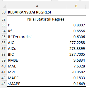
Model Goodness of Fit

Interpretation and Discussion:

1. Correlation Coefficient (r): An r value of 0.8097 indicates a strong relationship between the predictor variables and the response. This value is close to 1, signifying a strong and positive relationship.
2. Coefficient of Determination (R²): An R² value of 0.6556 means that approximately 65.56% of the variation in the response can be explained by this regression model.
3. Adjusted R²: An adjusted R² value of 0.6306 takes into account the number of predictors in the model and provides a more accurate estimate of how well the model will predict new samples.
4. AIC, AICc, and BIC: These are information criteria used to compare the relative quality of statistical models. A model with lower AIC, AICc, or BIC values is considered better. In this context, the AIC is 277.2288, AICc is 278.3399, and BIC is 287.7005.
5. RMSE (Root Mean Square Error): An RMSE value of 9.6834 indicates the average error between the observed values and the values predicted by the model. The lower the RMSE value, the better the model at predicting data.
6. MAE (Mean Absolute Error): An MAE value of 7.6328 indicates the average absolute error between the observed and predicted values. The lower the MAE value, the better the model.
7. MPE (Mean Percentage Error): An MPE value of -0.0582 indicates the average percentage error. A negative value suggests that the predictions tend to underestimate the actual values.
8. MAPE (Mean Absolute Percentage Error): A MAPE value of 0.1833 (or 18.33%) indicates the average absolute error in percentage terms.
9. sMAPE (symmetric Mean Absolute Percentage Error): An sMAPE value of 0.1649 (or 16.49%) is another measure of prediction error in percentage terms. It gives equal penalties for overestimation and underestimation, unlike MAPE.

From the above statistics, it can be concluded that the regression model has a fairly good fit, with some areas that may require further attention, such as prediction errors indicated by RMSE, MAE, and various other error metrics.

Regression Coefficient Estimates

From the table of regression coefficient estimates, here are the interpretations and discussions:

Interpretation and Discussion:

1. Intercept: The coefficient for the intercept is 25.259 with a standard deviation of 3.361. This indicates that if both fertilizer and compost doses are zero, the expected total dry weight would be approximately 25.259 grams per plant. With a 95% confidence level, the estimated interval for the intercept ranges from 18.523 to 31.995 grams.
2. Fertilizer Dose: The coefficient for fertilizer dose is 1.014 with a standard deviation of 0.163. This suggests that for each one-unit increase in fertilizer dose (assuming compost dose remains constant), the total dry weight would increase by approximately 1.014 grams. With a 95% confidence level, the estimated interval for this coefficient ranges from 0.688 to 1.341 grams. The t-statistic for this variable is 6.223, which is significant at the 1% level. The Variance Inflation Factor (VIF) for this variable is 12.252, indicating potential multicollinearity.
3. Fertilizer Dose^2: The coefficient for the quadratic effect of fertilizer dose is -0.011. This shows that there is a quadratic effect from the fertilizer dose on the total dry weight. With a 95% confidence level, the estimated interval for this coefficient ranges from -0.015 to -0.006. The t-statistic for this variable is -4.942, which is significant at the 1% level.
4. ... and so forth

From the above results, all variables in the model are significant in influencing the total dry weight at the 1% significance level. However, the relatively high VIF values for fertilizer and compost doses indicate the potential for multicollinearity, which can interfere with the interpretation of regression coefficients and reduce model reliability. Further analysis may be needed to address this issue.

3D Regression and Optimization Graph

Optimization methods aim to identify the optimal doses of fertilizer and compost that maximize the yield, in this case, the total dry weight of the plant. In mathematics, to find the maximum or minimum point of a function, differentiation techniques are used. By finding the point where the first derivative (differential) of the function is zero, we can determine the stationary points, which may be maximum, minimum, or inflection points. However, with SmartstatXL, this process has been simplified and can easily be performed with the help of statistical software.

Based on the regression model, to achieve the optimal total dry weight result (72.413), a combination of approximately 47.330-units of fertilizer dose and around 10.340 units of compost dose is required. On the other hand, without any fertilizer and compost application, the plant can still produce a dry weight of approximately 25.259 grams per plant.

Analysis of Variance (ANOVA) in Regression

Here are the interpretations and discussions from the ANOVA table:

Analysis of Variance (ANOVA):

1. Regression:
   • With 4 degrees of freedom (DF), the variance explained by the regression model is 9818.2471. The mean square (MS) for regression is 2454.5618.
   • The F-statistic for regression is 26.177, which is significant at the 1% level (P-Value = 0.000). This indicates that the regression model overall is significant in explaining the variance in total dry weight.
2. Fertilizer Dose:
   • The fertilizer dose accounts for a variance of 3631.7410 with an MS of 3631.7410.
   • The F-statistic for the fertilizer dose is 38.731, which is significant at the 1% level. This indicates that the fertilizer dose has a significant influence on the total dry weight.
3. ...and so on
4. Error:
   • The unexplained variance (error variance) is 5157.2428 with an MS of 93.7681.
   • Of this error variance, the model deviation contributes 1794.8294 with an MS of 119.6553, while the pure error contributes 3362.4133 with an MS of 84.0603.

Lack of Fit:

• Lack of Fit measures how well the constructed regression model fits the actual data. It indicates how much of the variance in the response is not explained by the regression model but could be explained by a more complex or appropriate model.
• From the table, the Lack of Fit has a variance of 1794.8294 with an MS of 119.6553.
• The F-statistic for Lack of Fit is 1.423, and with a P-Value of 0.184, the Lack of Fit is not significant at the 5% level. This means that the selected regression model does not show significant disagreement with the data, thereby making this model reasonably good in explaining the variance in the response.

Pure Error:

• Pure Error measures the natural variance or measurement errors present in the data. This is the variance that is truly unexplained by the model or any other factors.
• From the table, the Pure Error has a variance of 3362.4133 with an MS of 84.0603.
• This indicates that although the regression model has explained most of the variance in the response, there is still some unexplained variance due to either model deviation or natural variance/measurement errors.

Therefore, although the constructed regression model can explain most of the variance in total dry weight, there is still some variance caused by model deviation and natural variance or measurement errors. Both should be considered when assessing the reliability and accuracy of the model.

From the ANOVA analysis, it can be concluded that all predictor variables (fertilizer dose, quadratic effect of fertilizer dose, compost dose, and quadratic effect of compost dose) have a significant impact on the total dry weight at the 1% significance level. The constructed regression model is capable of explaining the variance in total dry weight well. However, there is still some unexplained variance, known as error variance.

Regression Assumption Checks

Normality and Heteroskedasticity Tests

Below are the interpretations and discussions from the Regression Assumption Checks:

1. Homoskedasticity Test:

• The Breusch-Pagan-Godfrey (BPG) test is performed to check the assumption of homoskedasticity in regression. Homoskedasticity means that the variance of the residuals (errors) should be constant across all levels of the predictor values.
• With 4 degrees of freedom (DF), the χ² test statistic for this test is 2.138 with a P-Value of 0.710.
• Since the P-Value > 0.05 (greater than 0.05), we fail to reject the null hypothesis. This means that the data meet the assumption of homoskedasticity, and there is no strong evidence of heteroskedasticity in the regression model.

2. Normality Test:

The Normality Test is performed to check the distribution of the residuals. The assumption is that the residuals should be normally distributed.

Based on the results from several Normality Tests:

• Shapiro-Wilk's: Statistic 0.983 with P-Value 0.587.
• Anderson Darling: Statistic 0.336 with P-Value 0.506.
• D'Agostino Pearson: Statistic 1.176 with P-Value 0.555.
• Liliefors: Statistic 0.074 with P-Value > 0.20.
• Kolmogorov-Smirnov: Statistic 0.074 with P-Value > 0.20.

All the Normality Tests indicate a P-Value greater than 0.05, which means we fail to reject the null hypothesis that the residuals are normally distributed. Therefore, the data meet the assumption of residual normality.

From the results of the Regression Assumption Checks, the constructed regression model meets the assumptions of homoskedasticity and residual normality. Both of these assumptions are crucial for ensuring the reliability and inferential validity of the regression model.

Residual Plots

In addition to formal tests, the assumption of normality can also be visually checked using the accompanying residual plots. Inspection can be done using the Normal Probability Plot (Normal P-Plot), Histogram, and Residual vs. Predicted Plot.

1. Normal P-Plot for Residuals:
   • The Normal Probability Plot between the residual values and the predicted or observed values. Ideally, the points on this plot should follow a straight diagonal line. If the points deviate from this diagonal line, it may indicate deviations from normality.
   • The fact that the points almost follow a straight diagonal line suggests that the residuals have a distribution that approximates normality across most value ranges. This is a good sign and indicates that the assumption of residual normality is largely met. However, the presence of points that deviate from the diagonal line at both ends indicates some deviation from normality in the tails of the distribution.
   • Although there are some deviations from normality, depending on the context and purpose of the analysis, these deviations may not be significant. However, if the analysis is highly sensitive to the assumption of normality, we may need to consider transformation techniques or other methods to correct these deviations.
2. Histogram for Residuals:
   • The Histogram should show a distribution that approximates a bell-shaped curve (normal distribution). Deviations from this shape (for example, a skewed or long-tailed distribution) may indicate a violation of the normality assumption.
3. Residual vs Predicted:
   • To check for homoskedasticity, the points on this plot should be randomly scattered around a horizontal line at 0 with no specific pattern. If a particular pattern is observed, such as a funnel shape or a curve, it may indicate heteroskedasticity or other violations of regression assumptions.

Given that all formal tests indicate that the residuals are normally distributed (as all p-values are greater than 0.05), the minor deviations on the Normal P-Plot are likely not a major concern.

In practice, regression analysis is often quite tolerant of minor violations of the normality assumption, especially if the sample size is sufficiently large. Therefore, even though there are some points that deviate from the diagonal line on the Normal P-Plot, if the formal tests indicate normality and we do not observe other significant violations of assumptions, the regression model may be considered sufficiently valid for analytical purposes.

Box-Cox Transformation and Residual Analysis

Below is the interpretation and discussion of the analysis results:

1. Box-Cox Transformation:
   • The Box-Cox Transformation is used to make the data more closely follow a normal distribution, especially if the data exhibits non-constant variance (heteroskedasticity) or is not normally distributed.
   • In this analysis, the lambda value obtained is 1.455. However, based on the information provided, no transformation is performed as it is stated "No Transformation: Y¹". This means that the original data (without transformation) satisfies the assumptions of the regression model.
2. Residual Values and Outlier Inspection:
   • Residuals are the differences between the observed values and the values predicted by the regression model.
   • Leverage indicates the extent to which individual observations influence the predictions made for them. High leverage values can indicate observations that have a significant impact on model estimation.
   • Studentized Residuals are standardized residuals. These residuals are useful for identifying outliers.
   • Studentized Deleted Residuals are similar to studentized residuals but are calculated by removing the concerned observation and estimating the model without it.
   • Cook's Distance measures the influence of individual observations on all other predictions. High values may indicate potentially high-influence observations.
   • DFITS is another measure of the influence of individual observations. Similar to Cook's Distance, but more focused on individual observations.

Checking residual values and outlier data is crucial in regression analysis. Outliers or observations with high influence can affect the reliability and interpretation of the regression model. Further consideration may be needed on how to handle these observations, whether to include them in the model or not.

Conclusion

1. The polynomial regression model generated from the analysis indicates that the fertilizer dose and compost dose have a significant effect on the total dry weight. The quadratic effects of both predictors are also significant.
2. The regression model successfully explains approximately 65.56% of the variation in total dry weight.
3. Based on the analysis of variance, all predictor variables have a significant effect on total dry weight at a significant level of 1%.
4. Regression assumptions such as homoskedasticity and residual normality are met based on the Breusch–Pagan–Godfrey test and Normality Tests.
5. From the Box-Cox transformation analysis, the data does not require transformation to meet the assumptions of regression.
6. Some observations may be outliers or have a high influence on the model based on the analysis of residual values and outlier inspection.

Reporting Results and Discussion in Scientific Papers

In this study, polynomial regression analysis was conducted with the response variable being the total dry weight (g/plant) against fertilizer and compost doses. From the analysis, a polynomial regression model was obtained indicating that fertilizer and compost doses have a significant impact on the total dry weight. This model successfully accounts for approximately 65.56% of the variation in total dry weight.

Based on the analysis of variance, all predictor variables were proven to have a significant effect on the total dry weight at a 1% significance level. Additionally, fundamental regression assumptions such as homoskedasticity and residual normality were met, indicating the validity of the resulting model.

In the initial stages of the analysis, a Box-Cox transformation check was conducted to ensure that the data meet the regression assumptions. The results showed that the data do not require further transformation. However, during the analysis process, some observations were found that may act as outliers or have a high influence on the model.

Conclusion:

Fertilizer and compost doses have a significant impact on the total dry weight of the plant. The resulting regression model is valid and meets the basic assumptions of regression. However, some observations may require further attention due to their potential as outliers or having a high influence on the model.